Pontryagin Dual
The goal of this section is to develop the representation theory of the compact group \[
\mathbb{T}= \operatorname{U}(1) \coloneqq \{ z \in \mathbb{C}: |z| = 1 \}.
\] Because \(\mathbb{T}\) is abelian, we know all its irreducible representations must one \(1\)-dimensional. In other words, studying the representation theory of \(\mathbb{T}\) is about understanding the space of homomorphisms \(\mathbb{T}\to \mathbb{T}\), just as it was for studying any finite abelian group \(A\). This sort of construction is so important that it earns its own name.
Definition 11.1 If \(A\) is a locally compact abelian group, we define \[
\widehat{A} \coloneqq \operatorname{Hom}(A,\mathbb{T})
\] as the Pontryagin dual group of \(A\). This set is a group under pointwise multiplication, i.e. the tensor product. Indeed, given continuous homomorphisms \(\rho, \sigma: A \to \mathbb{T}\) the map \[
g \mapsto (\rho \otimes \sigma)(g) = \rho(g) \sigma(g)
\] is also a continuous homomorphism \(A \to \mathbb{T}\). Moreover, we see that \(\rho^{-1}\) (as in, its inverse with respect to \(\otimes\), not its inverse as a map, which need not make sense) is the function \[
g \mapsto \overline{\rho(g)}.
\]
It turns out that, for a finite abelian group, we always have \(\widehat{A} \cong A\) (though the isomorphism is not natural). We will see that this is not the case for \(\mathbb{T}\). Moreover, the dual is so named because there is a natural isomorphism \[
A \to \skew{5.5}\widehat{\widehat{A}} \quad \text{ given by } \quad g \mapsto (\chi \mapsto \chi(g))
\] whenever \(A\) is a locally compact abelian group.
Example 11.1 Consider \(G = \mathbb{Z}/{3}\mathbb{Z}\), which has the irreducible representations (characters) \[
\chi_j: \mathbb{Z}/{3}\mathbb{Z} \to \mathbb{T}\quad \text{ given by } \chi_j(1) = e^{\tfrac{2\pi j}{3} i}
\] for \(0 \leq j < 3\). We have the multiplication table: \[
\begin{array}{r|ccc}
\widehat{\mathbb{Z}/{3}\mathbb{Z}} & \chi_0 & \chi_1 & \chi_2 \\ \hline
\chi_0 & \chi_0 & \chi_1 & \chi_2 \\
\chi_1 & \chi_1 & \chi_2 & \chi_0 \\
\chi_2 & \chi_2 & \chi_0 & \chi_1 \\
\end{array}
\] from which we can see an isomorphism \(\mathbb{Z}/{3}\mathbb{Z} \to \widehat{\mathbb{Z}/{3}\mathbb{Z}}\) via \(j \mapsto \chi_j\). Note that instead defining \(j \mapsto \chi_{2j}\) also gives an isomorphism between these groups and that there is no natural reason to prefer one isomorphism over the other.
Path Lifting
Remember that we want to understand the group \(\widehat{\mathbb{T}} \coloneqq \operatorname{Hom}(\mathbb{T},\mathbb{T})\). Our proof will rely on two workhorse Lemmas. The first is a formalization of Example 10.12:
Lemma 11.1 Any continuous homomorphism \(\rho: \mathbb{R}\to \mathbb{R}\) is of the form \[
\rho(t) = \lambda t
\] for some \(\lambda \in \mathbb{R}\). In other words, there is a bijection \(\operatorname{Hom}(\mathbb{R},\mathbb{R}) \longleftrightarrow \mathbb{R}\).
Proof. Given \(\rho: \mathbb{R}\to \mathbb{R}\), we define \(\lambda = \rho(1)\). Since homomorphisms send inverses to inverses, it follows that \(\rho(-1) = - \lambda\) and we also deduce \(\rho(n) = \lambda n\) for all \(n \in \mathbb{Z}\). Then we have \[
\rho(1) = \rho(\underbrace{\tfrac{1}{m} + \cdots + \tfrac{1}{m}}_m) = m \rho(\tfrac{1}{m}),
\] so we see that \(\rho(\tfrac{1}{m}) = \lambda \tfrac{1}{m}\) for all \(m \in \mathbb{Z}^+\). We can write any rational as \(\tfrac{n}{m}\) for \(n \in \mathbb{Z}\) and \(m \in \mathbb{Z}^+\), so we have \(\rho(\tfrac{n}{m}) = \lambda \tfrac{n}{m}\) by a similar argument. Hence, by the density of \(\mathbb{Q}\) in \(\mathbb{R}\) and continuity of \(\rho\) (c.f. Proposition 10.3), we see that \(\rho(t) = \lambda t\) for all \(t \in \mathbb{R}\).
Our second important lemma, whose proof is blackboxed for technical reasons but is conceptually quite intuitive, concerns the continuous homomorphism \(\epsilon: \mathbb{R}\to \mathbb{T}\) that winds the real line around the circle via \(\epsilon(t) = e^{it}\).
This map is quite nice; topologists call it a covering map, though we will not develop that language here. Even though this map is not injective—the kernel is \(2\pi \mathbb{Z}\subset \mathbb{R}\), which means every fiber is countably infinite—it enjoys the following property. Consider a connected open subarc of the circle, e.g., the set \[
U = \{ z \in \mathbb{T}: \Re(z)>0 \}.
\] The preimage of this set, \(\epsilon^{-1}(U)\), consists of infinitely many disjoint open intervals, \[
\epsilon^{-1}(U) = \bigcup_{n \in \mathbb{Z}} (\tfrac{4n-1}{2}\pi,\tfrac{4n+1}{2}\pi),
\] each of which is homeomorphic to \(U\) via the map \(\epsilon\). As a topologist might say, “\(\epsilon^{-1}(U)\) is a stack of pancakes over \(U\).” This is very neat, as it allows for the following construction.
Lemma 11.2 (Hatcher 2002, 29; Munkres 2000, 338) Every continuous map \(f: \mathbb{R}\to \mathbb{T}\) can be lifted to a continuous map \(\tilde{f}: \mathbb{R}\to \mathbb{R}\), i.e., there exists a function \(\tilde{f}\) such that \(\epsilon \circ \tilde{f} = f\):
While many lifts are possible, they are unique in the sense that, if there is another lift \(\bar{f}\) of \(f\) such that \(\tilde{f}(t_0) = \bar{f}(t_0)\) for some \(t_0 \in \mathbb{R}\), then \(\tilde{f}(t) = \bar{f}(t)\) for all \(t \in \mathbb{R}\).
We construct \(\tilde{f}\) as follows. Picking a starting point, say \(t=0\), and choose a point in the fiber over \(f(0)\) to be \(\tilde{f}(0)\). By choosing a small open arc \(U\) around \(f(0)\), the pre-image \(\epsilon^{-1}(U)\) is a stack of pancakes (in the sense above) over \(U\) where exactly one of the pancakes (call it \(U' \subset \mathbb{R}\)) contains \(\tilde{f}(0)\). Since the restriction \(\epsilon: U' \to U\) is a homeomorphism, we can define \(\tilde{f}(t)\) near \(t=0\) as simply \[
\tilde{f}(t) = \epsilon^{-1}(f(t)),
\] by which we mean the unique point in \(U'\) that maps via \(\epsilon\) to \(f(t)\). This will work for a while, but we might eventually find that \(f(t)\) moves so far from \(f(0)\) that we need to leave \(U\). That’s fine: if we are headed out of \(U\), we can pause at some \(t=t_0\) and repeat the whole procedure using a new arc centered at \(f(t_0)\). We can repeat this to determine \(\tilde{f}\) at any point (to make the argument rigorous, one needs to appeal to the notion of compactness to know the process will stop). Uniqueness follows since, once we know which pancake we are lifting points into, we cannot suddenly jump to another pancake without introducing a discontinuity—they are disjoint, after all!—so two lifts that agree somewhere must agree everywhere.
Accepting the path lifting Lemma on faith, we can immediately prove the following:
Theorem 11.1 If a continuous map \(f: \mathbb{R}\to \mathbb{T}\) is also a homomorphism, then it has a unique lift \(\tilde{f}: \mathbb{R}\to \mathbb{R}\) that is also a homomorphism.
Proof. We know \(f(0) = 1\); we claim that the lift of \(f\) satisfying \(\tilde{f}(0) = 0\) is a homomorphism. Fix \(s \in \mathbb{R}\) and note that the two maps \[
t \mapsto \tilde{f}(t+s) \quad \text{ and } \quad t \mapsto \tilde{f}(t) + \tilde{f}(s)
\] are continuous lifts of the map \(t \mapsto f(t)f(s)\). Moreover, these lifts agree at \(t=0\) and so they must agree for all \(t \in \mathbb{R}\) by uniqueness of lifts! We conclude that \(\tilde{f}\) is a homomorphism.
Irreducible Representations
Next we deduce a key Lemma, though it is important enough in and of itself to deserve the title of Theorem, on the way towards the desired result.
Theorem 11.2 Every continuous homomorphism \(f: \mathbb{R}\to \mathbb{T}\) is of the form \(f(t) = e^{\omega i t}\) for some \(\omega \in \mathbb{R}\). In other words, we have the parameterization \[
\operatorname{Hom}(\mathbb{R},\mathbb{T}) = \left\{ t \mapsto e^{\omega i t} \mid \omega \in \mathbb{R}\right\}.
\]
Proof. Given \(f: \mathbb{R}\to \mathbb{T}\), we lift to a homomorphism \(\tilde{f}: \mathbb{R}\to \mathbb{R}\) which must be of the form \(\tilde{f}(t) = \omega t\) for some \(\omega \in \mathbb{R}\) by Lemma 11.1. Therefore \[
f(t) = \epsilon( \tilde{f}(t) ) = \epsilon(\omega t) = e^{i \omega t}.
\]
In other words, the Pontryagin dual \(\widehat{\mathbb{R}}\) is \(\mathbb{R}\) itself.
We are ready to deduce \(\widehat{\mathbb{T}}\), i.e., the group that encodes all irreducible representations of \(\mathbb{T}\).
Theorem 11.3 We have the following parameterizations: \[
\begin{aligned}
\operatorname{Hom}(\mathbb{T},\mathbb{T}) & = \{ z \mapsto z^n : n \in \mathbb{Z}\} \\
\operatorname{Hom}(\mathbb{Z},\mathbb{T}) & = \{ k \mapsto z^k : z \in \mathbb{T}\}.
\end{aligned}
\] In other words, \(\widehat{\mathbb{T}} \cong \mathbb{Z}\) and, in turn, \(\widehat{\mathbb{Z}} \cong \mathbb{T}\).
Proof. Let \(f: \mathbb{T}\to \mathbb{T}\) be a continuous homomorphism. We remark that there are many such functions that we cannot lift to a map \(\mathbb{T}\to \mathbb{T}\); consider, for example, the identity map on \(\mathbb{T}\). On the other hand, we can lift the homomorphism \(h = f \circ \epsilon: \mathbb{R}\to \mathbb{T}\) to a homomorphism \(\tilde{h}: \mathbb{R}\to \mathbb{R}\) by Theorem 11.1. We have the commutative diagram:
\[
\begin{CD}
\mathbb{R}@>\tilde{h}>> \mathbb{R}\\
@V{\epsilon}VV @VV{\epsilon}V \\
\mathbb{T}@>>f> \mathbb{T}
\end{CD}
\]
Hence we know that \(\tilde{h}(t) = \lambda t\) for some \(\lambda \in \mathbb{R}\), from which we deduce \[
e^{i \lambda t} = f(e^{i t}).
\] Setting \(z = e^{i t}\), we have shown \(f(z) = z^\lambda\). Notice, however, that not every choice of \(\lambda\) yields a well-defined homomorphism \(f: \mathbb{T}\to \mathbb{T}\)! We must have \[
1 = e^{\lambda 0 i} = f(e^{0i}) = f(e^{2\pi i}) = e^{\lambda 2 \pi i} \not = 1 \text{ if } \lambda \not \in \mathbb{Z}.
\] Indeed, we can only have \(\lambda = n \in \mathbb{Z}\) for this map to make sense and, on the other hand, all such choices make for a continuous homomorphism \(\mathbb{T}\to \mathbb{T}\).
The second claim of the theorem requires no topology, since \(\mathbb{Z}\) is discrete as a subspace of \(\mathbb{R}\). Any homomorphism \(\mathbb{Z}\to \mathbb{T}\) is determined by where it sends \(1\) and any \(z \in \mathbb{T}\) is an allowable choice, since there are no relations on \(1 \in \mathbb{Z}\). Hence we get a distinct element in \(\mathbb{T}\) for every \(f \in \operatorname{Hom}(\mathbb{Z},\mathbb{T})\) by evaluating at \(1\), establishing the desired isomorphism.
Fourier Theory
We begin by rephrasing our main result from the previous section:
Theorem 11.4 Every irreducible representation of \(\mathbb{T}\) is of the form \[
\begin{aligned}
\rho_n: \mathbb{T}& \to \mathbb{T}\subset \operatorname{GL}_1(\mathbb{C}) \\
z & \mapsto z^n
\end{aligned}
\] for some \(n \in \mathbb{Z}\). We denote \(\mathbb{C}\) equipped with this action by \(U_n\), so any \(\mathbb{T}\)-representation \(V\) can be written as \[
V = \bigoplus_{k \in \mathbb{Z}} U_k^{\oplus a_k}
\] for a unique sequence of multiplicities \(a_k\) with only finitely many nonzero.
To avoid confusion, even though the two functions are identical because all representations involved are 1-dimensional, when thinking of \(\rho_n\) as a character we will denote it by \(\chi_n\).
As in Example 10.17, the Haar integral on \(\mathbb{T}= \operatorname{U}(1)\) is given by \[
f \mapsto \frac{1}{2\pi} \int_{0}^{2\pi} f(\theta) \mathop{}\!\mathrm{d}{\theta},
\] where we parameterize the circle by angle. This induces the inner product \[
\langle f_1, f_2 \rangle = \frac{1}{2\pi} \int_{0}^{2\pi} \overline{f_1(\theta)} f_2(\theta) \mathop{}\!\mathrm{d}{\theta},
\tag{11.1}\] for functions \(f_1, f_2 \in C^{}(\mathbb{T})\). Recall the orthogonality formula (Theorem 10.5) that we proved in a general setting for compact groups. In this context, it works out as the following: \[
\langle \chi_n, \chi_m \rangle = \frac{1}{2\pi} \int_0^{2\pi} \overline{\chi_n(\theta)} \chi_m(\theta) \mathop{}\!\mathrm{d}{\theta} = \frac{1}{2\pi} \int_0^{2\pi} e^{\theta(m-n)i} \mathop{}\!\mathrm{d}{\theta} = \left\{ \begin{array}{ll}
1 & \text{if } m = n \\
0 & \text{otherwise.}
\end{array} \right.
\] Given a representation \(V\) of \(\mathbb{T}\), we can use this orthogonality relationship just as we did for finite groups in order to deduce the multiplicities \(a_k\) of each irreducible \(U_k\) in \(V\). Remember, this decomposition is equivalent to finding coefficients \(a_k\) so that \[
\chi_V(\theta) = \sum_{k \in \mathbb{Z}} a_k e^{\theta k i},
\] so often we (or our favorite integration software) can use trigonometric identities, rather than integrals, in order to compute the desired multiplicities.
Example 11.2 Consider the representation \(\rho: \mathbb{T}\to \operatorname{GL}(V) = \operatorname{GL}_2(\mathbb{C})\) given by \[
\rho(\theta) = \begin{pmatrix}
5 \sin 2\theta + \cos 2\theta & -4 \sin \theta \cos \theta \\
26 \sin \theta \cos \theta & \cos 2\theta - 5 \sin 2\theta
\end{pmatrix}
\] The trace is given by \(\chi_V(\theta) = 2 \cos 2\theta\). So, on the one hand, we can compute integrals to deduce multiplicities—we’ll know that we are done when we find two dimensions worth of irreducible subrepresentations. For example: \[
\begin{gathered}
\langle \chi_0, \chi_V \rangle = \frac{1}{\pi} \int_0^{2\pi} \cos 2\theta \mathop{}\!\mathrm{d}{\theta} = 0 \quad \text{and} \quad \langle \chi_1, \chi_V \rangle = \frac{1}{\pi} \int_0^{2\pi} e^{-\theta i} \cos 2\theta \mathop{}\!\mathrm{d}{\theta} = 0, \\
\text{but} \quad \langle \chi_2, \chi_V \rangle = \frac{1}{\pi} \int_0^{2\pi} e^{-2\theta i} \cos 2\theta \mathop{}\!\mathrm{d}{\theta} = 1.
\end{gathered}
\] On the other hand, since \(e^{i2\theta} + e^{-i2\theta} = 2 \cos 2\theta\), we can conclude immediately that \(V = U_2 \oplus U_{-2}\).
Those practiced in the science of solving differential equations might call what we are doing by another name: we are computing the Fourier series of \(\chi_V\). This leads us to one of the difficulties that arises because of the infinitude of \(\mathbb{T}\): It is no longer true that we can write any class function \(\mathbb{T}\to \mathbb{C}\) as a linear combination of the characters \(\{\chi_n\}_{n \in \mathbb{Z}}\). Now we need to reconcile with infinite sums!
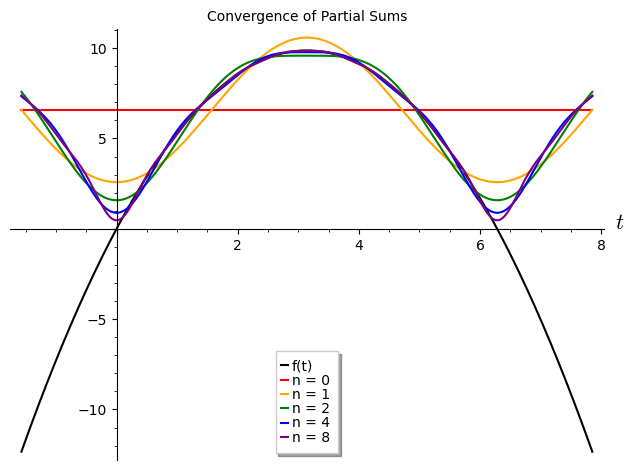
Example 11.3 Consider the function \(f(t) = t(2\pi - t)\) on the interval \([0,2\pi]\). We can compute \[
\begin{aligned}
a_0 & = \langle 1, f \rangle = \frac{4\pi^2}{3}, \\
a_k & = \langle \chi_k, f \rangle = \frac{1}{2\pi} \int_0^{2\pi} e^{-ikt} t(2\pi - t) \mathop{}\!\mathrm{d}{t} = - \frac{2}{k^2} \text{ for } k \not = 0,
\end{aligned}
\] and consider, say, the sequence of functions defined as the partial sums \[
s_n(t) \coloneqq \sum_{k = -n}^n a_k e^{ikt} = \frac{2\pi^2}{3} - \sum_{k=1}^n \frac{4}{k^2} \cos(kt)
\] as \(n \in \mathbb{N}\) grows to infinity. By consulting our favorite visualization software, we can see visually that at any \(t \in [0,2\pi]\) that \(s_n(t) \to f(t)\) as \(n\) grows to infinity.
Yet, at no point do we ever see an equivalence of functions \(s_n = f\) at any finite value for \(n\).
At work here is some analogy to our Theorem 8.1, where the characters of a finite group \(G\) constitute a basis for its vector space of class functions, with the added difficulties regarding convergence of functions.
Note that this process can be framed in terms of the Pontryagin dual: given \(f: A \to \mathbb{C}\), writing a class function in the orthonormal system of characters of \(A\) associates to \(f\) a scalar \(a_\xi\) as parameterized by \(\xi \in \hat{A}\). So the reason we obtain a sequence of numbers \((a_k)_{k \in \mathbb{Z}}\) from computing the Fourier series of a \(2\pi\)-periodic function \(f\) is because \(\hat{\mathbb{T}} \cong \mathbb{Z}\). If we instead consider functions \(f: \mathbb{R}\to \mathbb{C}\) with no periodicity condition, we instead arrive at what is more traditionally called the Fourier transform: \[
\mathscr{F}\{f\}(\omega) = \int_{-\infty}^\infty f(t) e^{-i\omega t} \mathop{}\!\mathrm{d}{t}.
\] This function of \(\omega \in \hat{\mathbb{R}} \cong \mathbb{R}\) is understood to describe the “frequencies” present in the original function.* The terms discrete Fourier transform and discrete-time Fourier transform are often used for the analogous transformation for functions on \(\mathbb{Z}/{n}\mathbb{Z}\) and \(\mathbb{Z}\), respectively.
We will not linger on these technical questions of convergence that are better answered in an analysis class, but mention that there are a number of well-studied sufficient conditions for the Fourier series of a function \(f: \mathbb{T}\to \mathbb{C}\) to converge at a given point \(\theta \in \mathbb{T}\), e.g., if \(f\) is differentiable at \(\theta\). Even jump discontinuities do not pose a serious problem, so long as the function is reasonably well-behaved to the left and right of the singularity!
In addition, there are also a number of useful theorems relating properties of a function and its Fourier series in favorable conditions, i.e., formulas like \[
\langle f, f \rangle = \sum_{k \in \mathbb{Z}} |a_k|^2,
\] which should remind us of Corollary 7.3.
Example 11.4 Consider \(\mathbb{T}\) parameterized by \(\theta \in (-\pi,\pi]\) and the function \[
f(\theta) = \left\{ \begin{array}{ll}
1 & \theta \geq 0 \\
-1 & \theta < 0,
\end{array} \right.
\] which has the Fourier coefficients \(a_{2k} = 0\) and \(a_{2k+1} = -\frac{2i}{\pi(2k+1)}\). The series converges to \(f(\theta)\) at each \(\theta \in (-\pi,\pi]\) except at the discontinuity, where it converges to \(0\). In general, altering the values of a function at a finite set of points will not change its Fourier series.
Hatcher, A. 2002. Algebraic Topology. Algebraic Topology. Cambridge University Press.
Munkres, J. R. 2000. Topology. Featured Titles for Topology. Prentice Hall, Incorporated.